Work, Energy and Power Part-3

5.9 THE POTENTIAL ENERGY OF A SPRING

The spring force is an example of a variable force which is conservative. Fig. 5.7 shows a block attached to a spring and resting on a smooth horizontal surface. The other end of the spring is attached to a rigid wall. The spring is light and may be treated as massless. In an ideal spring, the spring force $F_s$ is proportional to $x$ where $x$ is the displacement of the block from the equilibrium position. The displacement could be either positive [Fig. 5.7 (b)] or negative [Fig. 5.7(c)]. This force law for the spring is called Hooke’s law and is mathematically stated as

$$ F_s=-k x $$

The constant $k$ is called the spring constant. Its unit is $\mathrm{N} \mathrm{m}^{-1}$. The spring is said to be stiff if $k$ is large and soft if $k$ is small.

Suppose that we pull the block outwards as in Fig. 5.7 (b). If the extension is $x_m$, the work done by the spring force is

$$ \begin{aligned} W_s & =\int_0^{x_m} F_s \mathrm{~d} x=-\int_o^{x_m} k x \mathrm{~d} x \ & =-\frac{k x_m^2}{2}\hspace{60mm}(5.15) \end{aligned} $$

This expression may also be obtained by considering the area of the triangle as in Fig. 5.7(d). Note that the work done by the external pulling force $F$ is positive since it overcomes the spring force.

$$ \begin{equation*} W=+\frac{k x_{m}^{2}}{2} \tag{5.16} \end{equation*} $$

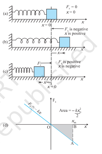
Fig. 5.7 Illustration of the spring force with a block attached to the free end of the spring. (a) The spring force $F_*$ is zero when the displacement $x$ from the equilibrium position is zero. (b) For the stretched spring $x>0$ and $F<0$ (c) For the compressed spring $x<0$ and $F_s>0$.(d) The plot of $F_3$ versus $x$. The area of the shaded triangle represents the work done by the spring force. Due to the opposing signs of $F_s$ and $x$, this work done is negative, $W_s=-k x_m^2 / 2$.

The same is true when the spring is compressed with a displacement $x_{c}(<0)$. The spring force does work $W_{s}=-k x_{c}^{2} / 2$ while the external force $F$ does work $+k x_{c}^{2} / 2$. If the block is moved from an initial displacement $x_{i}$ to a final displacement $x_{f}$, the work done by the spring force $W_{s}$ is

$$ W_s = -\int_{x_i}^{x_f} k x \,\mathrm{d}x = \frac{k x_i^2}{2} – \frac{k x_f^2}{2} \tag{5.17} $$

Thus the work done by the spring force depends only on the end points. Specifically, if the block is pulled from $x_i$ and allowed to return to $x_i$:

$$ \begin{aligned} W_s &= -\int_{x_i}^{x_i} k x \,\mathrm{d}x = \frac{k x_i^2}{2} – \frac{k x_i^2}{2} \\ &= 0 \end{aligned} \tag{5.18} $$

The work done by the spring force in a cyclic process is zero. We have explicitly demonstrated that the spring force (i) is position dependent only as first stated by Hooke, ( $F_s=-k x$ ); (ii) does work which only depends on the initial and final positions, e.g. Eq. (5.17). Thus, the spring force is a conservative force.

We define the potential energy $V(x)$ of the spring to be zero when block and spring system is in the equilibrium position. For an extension (or compression) $x$ the above analysis suggests that

$$ V(x)=\frac{k x^2}{2}\tag{5.19} $$

You may easily verify that $-\mathrm{d} V / \mathrm{d} x=-k x$, the spring force. If the block of mass $m$ in Fig. 5.7 is extended to $x_{m}$ and released from rest, then its total mechanical energy at any arbitrary point $x$, where $x$ lies between $-x_{m}$ and $+x_{m}$, will be given by

$$ \frac{1}{2} k x_{m}^{2}=\frac{1}{2} k x^{2}+\frac{1}{2} m v^{2} $$

where we have invoked the conservation of mechanical energy. This suggests that the speed and the kinetic energy will be maximum at the equilibrium position, $x=0$, i.e.,

$$ \frac{1}{2} m v_{m}^{2}=\frac{1}{2} k x_{m}^{2} $$

where $v_{m}$ is the maximum speed.

or $\quad v_{m}=\sqrt{\frac{k}{m}} x_{m}$

Note that $k / m$ has the dimensions of $\left[\mathrm{T}^{-2}\right]$ and our equation is dimensionally correct. The kinetic energy gets converted to potential energy and vice versa, however, the total mechanical energy remains constant. This is graphically depicted in Fig. 5.8.

Fig. 5.8 Parabolic plots of the potential energy V and kinetic energy K of a block attached to a spring obeying Hooke’s law. The two plots are complementary, one decreasing as the other increases. The total mechanical energy E = K + V remains constant

Example 5.8 To simulate car accidents, auto manufacturers study the collisions of moving cars with mounted springs of different spring constants. Consider a typical simulation with a car of mass 1000 kg moving with a speed $18.0 \ \mathrm{km} \ \mathrm{h}^{-1}$ on a smooth road and colliding with a horizontally mounted spring of spring constant $5.25 \times 10^3 \ \mathrm{N} \ \mathrm{m}^{-1}$. What is the maximum compression of the spring?

Answer: At maximum compression, the kinetic energy of the car is converted entirely into the potential energy of the spring.

The kinetic energy of the moving car is

$$ \begin{aligned} K &= \frac{1}{2} m v^2 \\ &= \frac{1}{2} \times 10^3 \times 5 \times 5 \\ &= 1.25 \times 10^4 \ \mathrm{J} \end{aligned} $$

where we have converted $18 \ \mathrm{km} \ \mathrm{h}^{-1}$ to $5 \ \mathrm{m} \ \mathrm{s}^{-1}$. It is useful to remember that $36 \ \mathrm{km} \ \mathrm{h}^{-1} = 10 \ \mathrm{m} \ \mathrm{s}^{-1}$.

At maximum compression $x_m$, the potential energy $V$ of the spring is equal to the kinetic energy $K$ of the moving car from the principle of conservation of mechanical energy:

$$ \begin{aligned} V &= \frac{1}{2} k x_m^2 \\ &= 1.25 \times 10^{4} \ \mathrm{J} \end{aligned} $$

We obtain $x_m = 2.00 \ \mathrm{m}$.

We note that we have idealised the situation. The spring is considered to be massless, and the surface has been considered to possess negligible friction.

We conclude this section by making a few remarks on conservative forces:

(i) Information on time is absent from the above discussions. In the example considered above, we can calculate the compression, but not the time over which the compression occurs. A solution of Newton’s Second Law for this system is required for temporal information.

(ii) Not all forces are conservative. Friction, for example, is a non-conservative force. The principle of conservation of energy will have to be modified in this case. This is illustrated in Example 5.9.

(iii) The zero of the potential energy is arbitrary. It is set according to convenience. For the spring force we took $V(x) = 0$ at $x = 0$, i.e., the unstretched spring had zero potential energy. For the constant gravitational force $mg$, we took $V = 0$ on the Earth’s surface. In a later chapter we shall see that for the force due to the universal law of gravitation, the zero is best defined at an infinite distance from the gravitational source. However, once the zero of the potential energy is fixed in a given discussion, it must be consistently adhered to throughout the discussion. You cannot change horses in midstream!

Example 5.9 Consider Example 5.8 taking the coefficient of friction, $\mu$, to be 0.5 and calculate the maximum compression of the spring.

Answer In presence of friction, both the spring force and the frictional force act so as to oppose the compression of the spring as shown in Fig. 5.9.

Fig. 5.9 The forces acting on the car.

We invoke the work-energy theorem, rather than the conservation of mechanical energy.

The change in kinetic energy is

$$ \Delta K=K_f-K_{\mathrm{i}}=0-\frac{1}{2} m v^2 $$

The work done by the net force is

$$ W=-\frac{1}{2} k x_m^2-\mu m g x_m $$

Equating we have

$$ \frac{1}{2} m v^2=\frac{1}{2} k x_m^2+\mu m g x_m $$

Now $\mu \mathrm{mg}=0.5 \times 10^3 \times 10=5 \times 10^3 \mathrm{~N}$ (taking $g=10.0 \mathrm{~m} \mathrm{~s}^{-2}$ ). After rearranging the above equation we obtain the following quadratic equation in the unknown $x_m$.

$$ \begin{aligned} & k x_m^2+2 \mu m g x_m-m v^2=0 \ & x_m=\frac{-\mu m g+\left[\mu^2 m^2 g^2+m k v^2\right]^{1 / 2}}{k} \end{aligned} $$

where we take the positive square root since $x_m$ is positive. Putting in numerical values we obtain

$$ x_m=1.35 \mathrm{~m} $$

which, as expected, is less than the result in Example 5.8.

If the two forces on the body consist of a conservative force $F_c$ and a non-conservative force $F_{n c}$, the conservation of mechanical energy formula will have to be modified. By the WE theorem

$$ \begin{gathered} \left(F_c+F_{n c}\right) \Delta x=\Delta K \ F_c \Delta x=-\Delta V \ \Delta(K+V)=F_{n c} \Delta x \ \Delta E=F_{n c} \Delta x \end{gathered} $$

But Hence, where $E$ is the total mechanical energy. Over the path this assumes the form

$$ E_f-E_i=W_{n c} $$

where $W_{n c}$ is the total work done by the non-conservative forces over the path. Note that unlike the conservative force, $W_{n c}$ depends on the particular path $i$ to $f$.

5.10 POWER

Often it is interesting to know not only the work done on an object, but also the rate at which this work is done. We say a person is physically fit if he not only climbs four floors of a building but climbs them fast. Power is defined as the time rate at which work is done or energy is transferred.

The average power of a force is defined as the ratio of the work, $W$, to the total time $t$ taken

$$ P_{a v}=\frac{W}{t}\hspace{35mm}(5.20) $$

The instantaneous power is defined as the limiting value of the average power as time interval approaches zero,

$$ P=\frac{\mathrm{d} W}{\mathrm{~d} t} $$

The work $d W$ done by a force F for a displacement $d \mathbf{r}$ is $\mathrm{d} W=\mathbf{F} . d \mathbf{r}$. The instantaneous power can also be expressed as

$$ \begin{aligned} & P=\mathbf{F} \cdot \frac{\mathrm{d} \boldsymbol{r}}{\mathrm{~d} t} \ & =\mathbf{F} \cdot \mathbf{v}\hspace{50mm}(5.21) \end{aligned} $$

where $\mathbf{v}$ is the instantaneous velocity when the force is $\mathbf{F}$.

Power, like work and energy, is a scalar quantity. Its dimensions are $\left[\mathrm{ML}^2 \mathrm{~T}^{-3}\right]$. In the SI, its unit is called a watt (W). The watt is $1 \mathrm{~J} \mathrm{~s}^{-1}$. The unit of power is named after James Watt, one of the innovators of the steam engine in the eighteenth century.

There is another unit of power, namely the horse-power (hp)

$$ 1 \mathrm{hp}=746 \mathrm{~W} $$

This unit is still used to describe the output of automobiles, motorbikes, etc.

We encounter the unit watt when we buy electrical goods such as bulbs, heaters and refrigerators. A 100 watt bulb which is on for 10 hours uses 1 kilowatt hour ( kWh ) of energy.

$$ \begin{aligned} & 100(\text { watt }) \times 10 \text { (hour) } \ & =1000 \text { watt hour } \ & =1 \text { kilowatt hour }(\mathrm{kWh}) \ & =10^3(\mathrm{~W}) \times 3600(\mathrm{~s}) \ & =3.6 \times 10^6 \mathrm{~J} \end{aligned} $$

Our electricity bills carry the energy consumption in units of $\mathrm{kWh}$. Note that $\mathrm{kWh}$ is a unit of energy and not of power.

Example 5.10 An elevator can carry a maximum load of $1800 \mathrm{~kg}$ (elevator + passengers) is moving up with a constant speed of $2 \mathrm{~m} \mathrm{~s}^{-1}$. The frictional force opposing the motion is 4000 N. Determine the minimum power delivered by the motor to the elevator in watts as well as in horse power.

Answer The downward force on the elevator is

$$ F=m g+F_{f}=(1800 \times 10)+4000=22000 \mathrm{~N} $$

The motor must supply enough power to balance this force. Hence,

$$ P=\mathbf{F} \cdot \mathbf{v}=22000 \times 2=44000 \mathrm{~W}=59 \mathrm{hp} $$

5.11 COLLISIONS

In physics we study motion (change in position). At the same time, we try to discover physical quantities, which do not change in a physical process. The laws of momentum and energy conservation are typical examples. In this section we shall apply these laws to a commonly encountered phenomena, namely collisions. Several games such as billiards, marbles or carrom involve collisions.We shall study the collision of two masses in an idealised form.

Consider two masses $m_1$ and $m_2$. The particle $m_1$ is moving with speed $v_{1 i}$, the subscript ’ $i$ ’ implying initial. We can cosider $m_2$ to be at rest. No loss of generality is involved in making such a selection. In this situation the mass $m_1$ collides with the stationary mass $m_2$ and this is depicted in Fig. 5.10.

The masses $m_{1}$ and $m_{2}$ fly-off in different directions. We shall see that there are relationships, which connect the masses, the velocities and the angles.

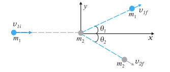
Fig. 5.10 Collision of mass m1 , with a stationary mass m2 .

5.11.1 Elastic and Inelastic Collisions

In all collisions the total linear momentum is conserved; the initial momentum of the system is equal to the final momentum of the system. One can argue this as follows. When two objects collide, the mutual impulsive forces acting over the collision time $\Delta t$ cause a change in their respective momenta :

$$ \begin{aligned} & \Delta \mathbf{p}_1 = \mathbf{F}_{12} \, \Delta t \\ & \Delta \mathbf{p}_2 = \mathbf{F}_{21} \, \Delta t \end{aligned} $$

where $ \mathbf{F}_{12} $ is the force exerted on the first particle by the second particle. $ \mathbf{F}_{21} $ is likewise the force exerted on the second particle by the first particle. Now from Newton’s third law, $\mathbf{F}_{12} = -\mathbf{F}_{21}$. This implies

$$ \Delta \mathbf{p}_1 + \Delta \mathbf{p}_2 = \mathbf{0} $$

The above conclusion is true even though the forces vary in a complex fashion during the collision time $\Delta t$. Since the third law is true at every instant, the total impulse on the first object is equal and opposite to that on the second.

On the other hand, the total kinetic energy of the system is not necessarily conserved. The impact and deformation during collision may generate heat and sound. Part of the initial kinetic energy is transformed into other forms of energy. A useful way to visualise the deformation during collision is in terms of a ‘compressed spring’. If the ‘spring’ connecting the two masses regains its original shape without loss in energy, then the initial kinetic energy is equal to the final kinetic energy but the kinetic energy during the collision time $\Delta t$ is not constant. Such a collision is called an elastic collision. On the other hand the deformation may not be relieved and the two bodies could move together after the collision. A collision in which the two particles move together after the collision is called a completely inelastic collision. The intermediate case where the deformation is partly relieved and some of the initial kinetic energy is lost is more common and is appropriately called an inelastic collision.

5.11.2 Collisions in One Dimension

Consider first a completely inelastic collision in one dimension. Then, in Fig. 5.10,

$$ \begin{align*} & \theta_{1}=\theta_{2}=0 \\ & m_{1} v_{1 i}=\left(m_{1}+m_{2}\right) v_{f} \text { (momentum conservation) } \\ & v_{f}=\frac{m_{1}}{m_{1}+m_{2}} v_{1 i} \tag{5.22} \end{align*} $$

The loss in kinetic energy on collision is

$$ \begin{aligned} & \Delta K=\frac{1}{2} m_{1} v_{1 i}^{2}-\frac{1}{2}\left(m_{1}+m_{2}\right) v_{f}^{2} \\ & =\frac{1}{2} m_{1} v_{1 i}^{2}-\frac{1}{2} \frac{m_{1}^{2}}{m_{1}+m_{2}} v_{1 i}^{2} \quad \text { [using Eq. (5.22)] } \\ & =\frac{1}{2} m_{1} v_{1 i}^{2} \left(1-\frac{m_{1}}{m_{1}+m_{2}}\right) \\ & =\frac{1}{2} \frac{m_{1} m_{2}}{m_{1}+m_{2}} v_{1 i}^{2} \end{aligned} $$

which is a positive quantity as expected.

Consider next an elastic collision. Using the above nomenclature with $\theta_{1}=\theta_{2}=0$, the momentum and kinetic energy conservation equations are

$$ \begin{align*} & m_{1} v_{1 i}=m_{1} v_{1 f}+m_{2} v_{2 f} \tag{5.23}\\ & m_{1} v_{1 i}^{2}=m_{1} v_{1 f}^{2}+m_{2} v_{2 f}^{2} \tag{5.24} \end{align*} $$

From Eqs. (5.23) and (5.24) it follows that,

$$ m_{1} v_{1 i}\left(v_{2 f}-v_{1 i}\right)=m_{1} v_{1 f}\left(v_{2 f}-v_{1 f}\right) $$

or,

$$ \begin{align*} v _{2 f}\left(v _{1 i}-v _{1 f}\right) & =v _{1 i}^{2}-v _{1 f}^{2} \\ & =\left(v _{1 i}-v _{1 f}\right)\left(v _{1 i}+v _{1 f}\right) \tag{5.25} \end{align*} $$

Substituting this in Eq. (5.23), we obtain

$$ \begin{align*} v_{1 f} & =\frac{\left(m_{1}-m_{2}\right)}{m_{1}+m_{2}} v_{1 i} \tag{5.26}\\ \text { and } \quad v_{2 f} & =\frac{2 m_{1} v_{1 i}}{m_{1}+m_{2}} \tag{5.27} \end{align*} $$

Thus, the ‘unknowns’ {$V_{1f} \quad V_{2f}$} are obtained in terms of the ‘knowns’ {$ m_1, m_2, v_1 i $}. Special cases of our analysis are interesting.

Case I : If the two masses are equal

$$ \begin{aligned} & V_{1 f}=0 \\ & V_{2 f}=V_{1 i} \end{aligned} $$

The first mass comes to rest and pushes off the second mass with its initial speed on collision.

Case II : If one mass dominates, e.g. $m_{2} > > m_{1}$

$$ V_{1 f} \simeq-V_{1 i} \quad V_{2 f} \simeq 0 $$

The heavier mass is undisturbed while the lighter mass reverses its velocity.

Example 5.11 Slowing down of neutrons: In a nuclear reactor a neutron of high speed (typically $10^7 \mathrm{~m} \mathrm{~s}^{-1}$ ) must be slowed to $10^3 \mathrm{~m} \mathrm{~s}^{-1}$ so that it can have a high probability of interacting with isotope ${ }_{92}^{235} \mathrm{U}$ and causing it to fission. Show that a neutron can lose most of its kinetic energy in an elastic collision with a light nuclei like deuterium or carbon which has a mass of only a few times the neutron mass. The material making up the light nuclei, usually heavy water $\left(\mathrm{D}_2 \mathrm{O}\right)$ or graphite, is called a moderator.

Answer The initial kinetic energy of the neutron is

$$ K_{1 i}=\frac{1}{2} m_{1} v_{1 i}^{2} $$

while its final kinetic energy from Eq. (5.26)

$$ K_{1 f}=\frac{1}{2} m_{1} v_{1 f}^{2}=\frac{1}{2} m_{1} \left(\frac{m_1-m_2}{m_1+m_2} \right)^{2} v_{1 i}^{2} $$

The fractional kinetic energy lost is

$$ f_{1}=\frac{K_{1 f}}{K_{1 i}}=\left(\frac{m_1-m_2}{m_1+m_2} \right)^{2} $$

while the fractional kinetic energy gained by the moderating nuclei $K_{2 f} / K_{l i}$ is

$$ \begin{aligned} f_{2}=1 & -f_{1} \text { (elastic collision) } \\ = & \frac{4 m_{1} m_{2}}{\left(m_{1}+m_{2}\right)^{2}} \end{aligned} $$

One can also verify this result by substituting from Eq. (5.27).

For deuterium $m_2=2 m_1$ and we obtain $f_1=1 / 9$ while $f_2=8 / 9$. Almost $90 %$ of the neutron’s energy is transferred to deuterium. For carbon $f_1=71.6 %$ and $f_2=28.4 %$. In practice, however, this number is smaller since head-on collisions are rare.

If the initial velocities and final velocities of both the bodies are along the same straight line, then it is called a one-dimensional collision, or head-on collision. In the case of small spherical bodies, this is possible if the direction of travel of body 1 passes through the centre of body 2 which is at rest. In general, the collision is two- dimensional, where the initial velocities and the final velocities lie in a plane.

5.11.3 Collisions in Two Dimensions

Fig. 5.10 also depicts the collision of a moving mass $m_1$ with the stationary mass $m_2$. Linear momentum is conserved in such a collision. Since momentum is a vector this implies three equations for the three directions ${x, y, z}$. Consider the plane determined by the final velocity directions of $m_1$ and $m_2$ and choose it to be the $x$–$y$ plane. The conservation of the $z$-component of the linear momentum implies that the entire collision is in the $x$–$y$ plane. The $x$- and $y$-component equations are

$$ \begin{aligned} & m_1 v_{1 i} = m_1 v_{1 f} \cos \theta_1 + m_2 v_{2 f} \cos \theta_2 \hspace{40mm} (5.28) \\ & 0 = m_1 v_{1 f} \sin \theta_1 – m_2 v_{2 f} \sin \theta_2 \hspace{48mm} (5.29) \end{aligned} $$

One knows $\{ m_1, m_2, v_{1 i} \}$ in most situations. There are thus four unknowns $\{ v_{1 f}, v_{2 f}, \theta_1, \theta_2 \}$, and only two equations. If $\theta_1 = \theta_2 = 0$, we regain Eq. (5.23) for one-dimensional collision. If, further, the collision is elastic,

$$ \frac{1}{2} m_1 v_{1 i}^2 = \frac{1}{2} m_1 v_{1 f}^2 + \frac{1}{2} m_2 v_{2 f}^2 \hspace{48mm} (5.30) $$

We obtain an additional equation. That still leaves us one equation short. At least one of the four unknowns, say $\theta_1$, must be made known for the problem to be solvable. For example, $\theta_1$ can be determined by moving a detector in an angular fashion from the $x$ to the $y$ axis. Given $\{ m_1, m_2, v_{1 i}, \theta_1 \}$ we can determine $\{ v_{1 f}, v_{2 f}, \theta_2 \}$ from Eqs. (5.28)–(5.30).

Example 5.12 Consider the collision depicted in Fig. 5.10 to be between two billiard balls with equal masses $m_{1} = m_{2}$. The first ball is called the cue while the second ball is called the target. The billiard player wants to “sink” the target ball in a corner pocket, which is at an angle $\theta_{2} = 37^\circ$. Assume that the collision is elastic and that friction and rotational motion are not important. Obtain $\theta_{1}$.

Answer From momentum conservation, since the masses are equal:

$$ \mathbf{v}_{1 i} = \mathbf{v}_{1 f} + \mathbf{v}_{2 f} $$

or,

$$ \begin{aligned} & v_{1 i}^2 = \left( \mathbf{v}_{1 f} + \mathbf{v}_{2 f} \right) \cdot \left( \mathbf{v}_{1 f} + \mathbf{v}_{2 f} \right) \\ & = v_{1 f}^2 + v_{2 f}^2 + 2 \mathbf{v}_{1 f} \cdot \mathbf{v}_{2 f} \end{aligned} $$

$$ = v_{1 f}^2 + v_{2 f}^2 + 2 v_{1 f} v_{2 f} \cos \left( \theta_1 + 37^\circ \right) \tag{5.31} $$

Since the collision is elastic and $m_{1} = m_{2}$, it follows from conservation of kinetic energy that

$$ v_{1 i}^{2} = v_{1 f}^{2} + v_{2 f}^{2} \tag{5.32} $$

Comparing Eqs. (5.31) and (5.32), we get

$$ \cos \left( \theta_{1} + 37^\circ \right) = 0 $$

$$ \text{or} \quad \theta_{1} + 37^\circ = 90^\circ $$

Thus, $\theta_{1} = 53^\circ$.

This proves the following result: when two equal masses undergo a glancing elastic collision with one of them at rest, after the collision, they will move at right angles to each other. The matter simplifies greatly if we consider spherical masses with smooth surfaces, and assume that collision takes place only when the bodies touch each other. This is what happens in the games of marbles, carrom, and billiards.

In our everyday world, collisions take place only when two bodies touch each other. But consider a comet coming from far distances to the Sun, or an alpha particle coming towards a nucleus and going away in some direction. Here we have to deal with forces involving action at a distance. Such an event is called scattering. The velocities and directions in which the two particles go away depend on their initial velocities as well as the type of interaction between them, their masses, shapes, and sizes.